
Calibration That Pays: Why Forecast “Accuracy” Fails Once Trading Costs Exist
A walk-forward study on S&P 500 futures shows that fixing probability reliability in the economically decisive regions reduces turnover tails, constraint binding, and realised decision loss—even when

Keywords
Calibration; transaction costs; market impact; walk-forward evaluation; decision loss; forecasting; market microstructure; turnover; constraints; futures; reliability diagrams; robustness; model risk; monitoring; financial econometrics.
Calibration That Pays: Why Forecast “Accuracy” Fails Once Trading Costs Exist
Forecasting in finance has an embarrassment built into it. We have a decade of increasingly sophisticated models—richer features, stronger algorithms, sharper validation—yet the moment you route those predictions through a real execution layer, the “best” model often stops being the best. Something mundane and brutal takes over: turnover, spreads, impact, and constraints. The model that wins on paper becomes the one that overtrades in reality.
This piece summarises a simple claim, tested in a pre-committed walk-forward design: when trading frictions and constraints exist, probabilistic calibration is not a diagnostic nicety. It is a decision-relevant object. Calibrating the forecast distribution—especially in the regions that actually move the optimiser—reduces the trading behaviours that destroy net performance.
The core finding is not that calibration makes forecasts “more accurate” in the usual sense. It’s that calibration makes decisions less wrong in the ways that matter under costs.
The problem: evaluation rewards the wrong thing
Most forecasting workflows in empirical finance still treat prediction as the end of the story. We compare models with point metrics—MSE, MAE, hit rates—and, if we’re being careful, we add a few probabilistic scores. Then we hand the “winner” to a portfolio rule and assume the portfolio will inherit the forecast superiority.
Execution does not behave that way. Execution punishes shape errors—overconfidence, mis-scaled tails, mis-ranked states—because those errors produce aggressive position changes precisely when liquidity is thin and the cost curve is steep. If a model is too sure of itself, the optimiser trades too much. If it misstates tail probabilities, it leans hard into rare states and gets clipped by constraints or by impact. The realised outcome is not “slightly worse”. It is qualitatively different, because convex costs and binding constraints turn small forecast distortions into big economic errors.
So the relevant metric is not point forecast loss. It is decision loss, measured after frictions and feasibility constraints.
In this study, the primary endpoint is realised decision loss defined as the negative of friction-adjusted return. Lower is better. It’s the thing you would actually care about if you were held accountable for implementation rather than for a tidy backtest.
The experiment: a walk-forward test with three configurations
The evaluation uses a pre-committed walk-forward protocol: the procedure is fixed before looking at the full run, and methods are compared on aligned timestamps. The sample is intentionally high-frequency because frictions are measurable only there.
Window: December 1–31, 2025
Horizon: minute-level decisions
Aligned decision periods: N = 8,025
Contracts: S&P 500 E-mini futures, rolling across ESZ5 (early December) and ESH6 (late December) per the dataset alignment.
Three configurations are compared:
Uncalibrated: baseline predictive distribution used as-is.
Standard Calibration: isotonic regression (a standard monotone calibration benchmark).
Utility-Weighted Calibration (UWC): a calibration warp that weights calibration errors by their economic relevance—specifically, by how much the optimiser’s decision and friction exposure respond to those errors.
Everything else is held fixed: decision rule, cost operator form, and constraints.
The primary result: UWC dominates on realised decision loss
Here is the chart that matters.
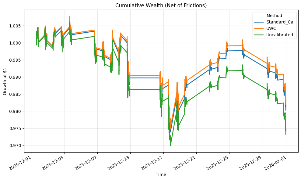
Insert: figures/fig_cumulative_wealth.png
This figure plots cumulative decision loss through time. Because decision loss is defined as the negative of friction-adjusted return, lower cumulative loss is better. What you see is not a one-off gap. It is a persistent divergence: UWC accumulates loss more slowly than the uncalibrated system, with the gap widening most in the stressier parts of the month.
The unconditional numbers are consistent with the chart. UWC has the lowest mean decision loss. Uncalibrated is worse. Standard calibration sits between them.
The deeper test is paired. Since all methods are evaluated on the same timestamps, we can look at the loss differential series:
Δₜ = loss(UWC) − loss(Uncalibrated)
This differential is negative on average—meaning UWC wins—and the mean differential is about −1.0×10⁻⁶ per minute with a t-statistic around −30.31 on the aligned sample. The magnitudes per minute look small because the horizon is small. The relevant quantity is the cumulative drift: a small negative mean per minute becomes economically meaningful at scale and is precisely the kind of effect that survives costs.
UWC also beats standard isotonic calibration, with a smaller but still clearly significant edge (t-stat about −6.63). That matters because it shows the contribution is not “calibration in general.” It’s the fact that the calibration objective is targeted to the decision mechanism.
If you remember one sentence: UWC dominates because it reduces the economic failure modes induced by miscalibrated uncertainty.
Calibration diagnostics: the mechanism is visible
If the first figure shows the effect, the reliability plot shows the cause.
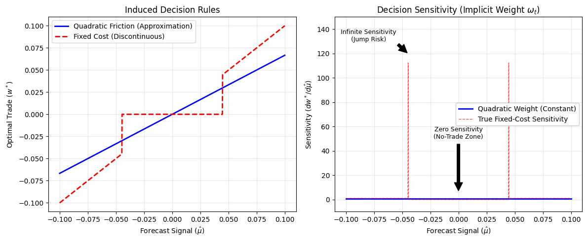
Insert: figures/fig_reliability_diagram.png
The uncalibrated method displays the classic S-shape: it assigns extreme probabilities far more often than the realised frequency supports. This is what overconfidence looks like in a reliability diagram. And in trading, overconfidence is not just a statistical sin. It is an operational command: “trade harder”.
UWC pulls the curve back toward the diagonal, especially where it matters. The point is not to make probabilities aesthetically pleasing. The point is that the optimiser reads those probabilities as inputs to position sizing and turnover decisions. Fixing the probability shape is how you stop the optimiser from manufacturing turnover out of noise.
Where performance is won or lost: turnover tails and corner solutions
Friction is not linear. In liquid markets you can pretend it is for a while, but once participation grows or volatility rises, the cost curve bends upward. That is where “accuracy” dies and implementation reality begins.
The key behaviour is turnover. Not average turnover in the centre of the distribution, but the right tail: the bursts where the model demands large position changes in a short time. Those bursts are where impact and binding constraints bite.
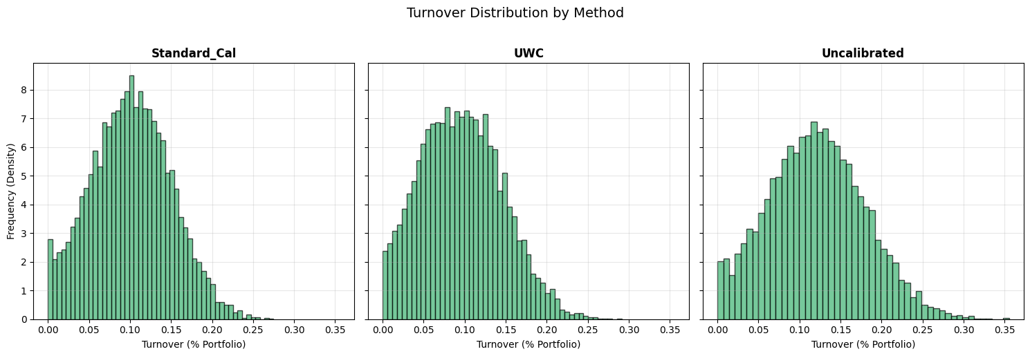
The turnover distribution makes this concrete. The uncalibrated system exhibits a heavy right tail—frequent high-turnover events. Even if the mean turnover difference looks modest, the tail matters disproportionately because convex costs punish the tail.
UWC compresses that right tail. It does not need to be clairvoyant. It needs to be less wrong in the regions where “wrong” means “trade a lot, right now”.
The constraint channel tells the same story. When the forecast is overconfident, it regularly asks for trades that exceed capacity or turnover limits. The optimiser is then forced into a corner: it truncates trades, reassigns turnover budget, and produces a realised portfolio that differs from the model-implied optimum. That is a structural failure: your forecast is no longer even being implemented.
UWC reduces the frequency of those corner events by producing uncertainty that scales positions down into feasibility. It keeps the optimiser in the interior more often, where the decision mapping is smoother and less brittle.
That is what “calibration is decision-relevant” means in practice: it is a control on the optimiser’s tendency to create high-cost events.
Robustness: sensitivity, placebos, and alternative objectives
A Substack piece does not need to replicate every table, but it must address the obvious objections.
Cost and capacity sensitivity
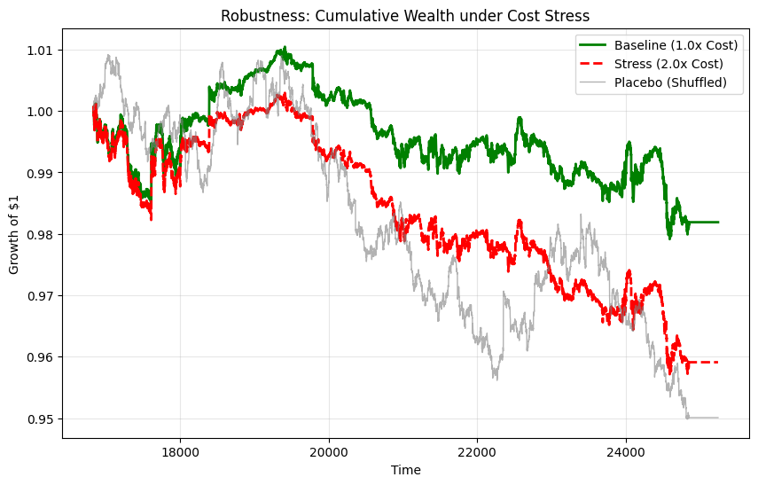
You ran sensitivity scenarios by scaling cost parameters and tightening capacity constraints. The pattern is what you would expect if frictions are the mechanism: as costs increase, net performance degrades, and constraint binding rises under tight caps. This is not a surprise; it is a falsifiable implication. If costs did not matter, cost scaling would not move results.
In other words: the conclusions are not a statistical artefact of a particular cost coefficient. They are about shape and behaviour under frictions.
Placebo checks (shuffled signals)
A shuffled-signal placebo is the simplest anti-leakage test: if the strategy still “works” under shuffled forecasts, you likely have timing issues, leakage, or a bookkeeping error. In your run, the placebo collapses (NaNs in performance metrics), which is consistent with “no genuine signal survives randomisation.” That is what you want to see.
Alternative objectives
The paper also considers risk-focused objectives such as CVaR(5%) and max drawdown. The numbers you computed show UWC improves drawdown relative to the uncalibrated baseline and remains competitive on CVaR. The important point is not that every metric changes dramatically; it is that the UWC advantage is not confined to a single choice of objective. If calibration matters via turnover tails and constraint corners, it should show up whenever the optimiser pays for aggressive rebalancing.
Alternative contracts within the same market
You also split results by contract symbol (ESZ5 vs ESH6). The dominance pattern persists in both segments. That matters because it reduces the chance that the entire effect is a quirk of a single contract or a single subperiod.
If you want to demonstrate generality beyond this paper, you add more months, not more adjectives. But within December 2025, the cross-contract check is the correct minimal robustness step.
Model risk and governance: why this belongs in econometrics, not just engineering
A strategy can look stable and still be fragile. Model risk is the difference between “works in-sample” and “survives stress”.
You constructed a model-risk set by perturbing:
the predictive distribution (mean drift; volatility regime shift), and
the cost environment (liquidity shock via cost multipliers),
then combining them to measure a worst-case expected decision loss.
The result is intuitive and sharp: under adverse selection (mean shift) the expected loss can jump by orders of magnitude; liquidity shocks are smaller but still material; the combined stress is the breaking point.
This is not merely a risk-management appendix. It is a formalisation: stress as optimisation—the worst-case loss over a neighbourhood around the forecast and/or cost parameters.
For monitoring, the governance chart provides the operational complement: a rolling drift statistic (standardised loss differential) and an intervention threshold (e.g., 2σ). In your run, the measured “model breakdown frequency” above the threshold is effectively zero. That does not prove permanence; it shows how the rule behaves in this window.
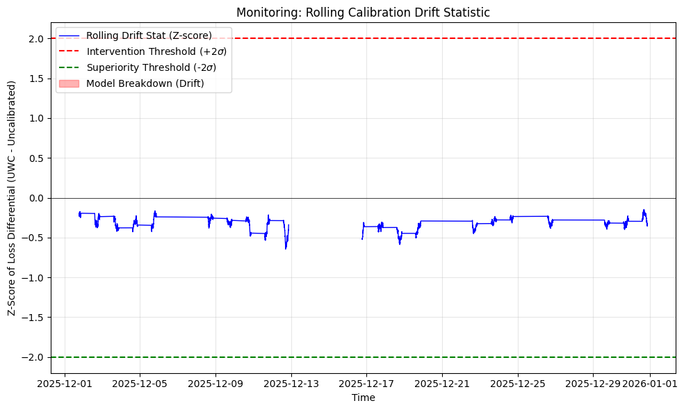
The reason this matters is discipline. If the method is to be taken seriously, it must come with a monitoring statistic that can be computed in production and a rule that tells you when to intervene. Otherwise it remains a clever calibration trick that no one can deploy responsibly.
Limitations: one month is not a regime, and it should be treated as such
The empirical evaluation is narrow in calendar time: December 1–31, 2025, minute horizon, N = 8,025. This narrowness is intentional because intraday frictions are measurable only at this frequency. But it does limit generality.
A single month cannot span the full regime space: protracted bull markets, persistent drawdowns, volatility compressions, crisis dislocations. It also increases exposure to microstructure quirks—contract roll mechanics, month-end effects, and temporary liquidity patterns. Pre-commitment mitigates some of the overfitting risk by fixing the evaluation procedure, but it does not abolish it.
So the honest interpretation is: this is a controlled demonstration that, in a real intraday friction environment, calibration aligned to decision sensitivity reduces turnover tails, constraint binding, and realised decision loss. The general claim requires replication across more months and more regimes with the same protocol discipline.
The takeaway: calibration is not decoration when costs exist
If you trade in a frictionless world, you can optimise forecasts for point accuracy and pretend the portfolio will take care of itself. In the world we live in, frictions and constraints make that fantasy expensive.
This research makes a measurable, operational claim:
A utility-weighted calibration warp can produce lower realised decision loss, net of costs and constraints, in a pre-committed walk-forward test.
The mechanism is visible: improved reliability in decision-relevant regions compresses turnover tails and reduces corner solutions.
The advantage is robust to cost scaling, alternative objectives, placebo checks, and contract segmentation within the tested month.
And it sets up the next step. Calibration is not end-to-end learning. It is a modular layer that makes the forecast distribution behave like a truthful input to an optimiser. The next paper—decision-focused learning under frictions—goes further: it trains the forecast and the policy together by optimising decision loss directly. That is a different philosophy, and it may yield further gains, but it is also more fragile, more expensive, and harder to govern.
A sensible sequence is exactly the one this work implies: make the probabilistic primitive reliable under frictions first; then decide whether end-to-end optimisation is worth the added complexity.