The Bipartite Shadow Hypothesis: Where Erdős–Hajnal Now Bottlenecks

From log–log bounds and pivot-minor structure to a single bipartite obstruction

Keywords / Tags

Erdős–Hajnal, Strong Erdős–Hajnal, Bipartite graphs, Hereditary classes, Induced , subgraphs, Chain graphs, Pivot-minors, P₆-free graphs, Extremal graph theory, Structural decomposition

---

1. Why Erdős–Hajnal Changed in the Last Five Years

For more than three decades, the Erdős–Hajnal conjecture was treated primarily as a problem of quantitative extremal bounds. Given a fixed forbidden induced subgraph ( H ), how large a clique or stable set must appear in an ( H )-free graph on ( n ) vertices? The conjecture predicts a polynomial bound; the reality, for most ( H ), stalled far below that threshold. Progress was measured in exponents and iterated logarithms, and the dominant techniques were global: Ramsey-type arguments, regularity, and density increments.

That framing has now shifted decisively.

What has become clear over the last five years is that the bottleneck in Erdős–Hajnal is not primarily numerical. It is structural. The hard cases are not those where one barely misses a polynomial bound, but those where the graph admits no obvious mechanism forcing large homogeneous structure at all. In response, the focus of the field has moved away from “how big a clique or stable set can we guarantee?” toward a sharper question: what local constraints force macroscopic homogeneity, and how can they be iterated?

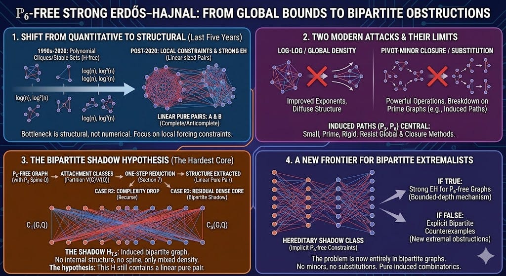
This shift is visible across multiple strands of recent work. The emergence of strong Erdős–Hajnal—the guarantee of linear-sized complete or anticomplete pairs—has provided a clearer structural target than cliques or stable sets alone. Pure pairs behave well under restriction, compose naturally in inductive arguments, and align more closely with decomposition-based reasoning. Once one insists on pure pairs, many traditional global techniques lose relevance, and local structure comes to the fore.

At the same time, there has been a growing recognition that many previously successful approaches relied, often implicitly, on substitution or modular decomposition. Those tools break down exactly when the forbidden graph is prime. Induced paths are the canonical example. A path has no nontrivial modules, and forbidding it does not impose obvious global density constraints. Any argument that hopes to resolve Erdős–Hajnal for induced paths must therefore be intrinsic to path structure itself, not inherited from closure properties.

This is why induced paths—especially ( P_5 ) and ( P_6 )—have become central. They are small, prime, and rigid enough to impose constraints, yet large enough to resist the usual shortcuts. Progress on these cases has exposed the limits of both global density methods and purely closure-based approaches. It has also clarified what a successful strategy must look like: one that replaces asymptotic counting with finite, checkable systems of constraints that propagate under restriction.

The present work is situated squarely within this newer perspective. It does not attempt to improve bounds by shaving exponents. Instead, it asks a different question: given a fixed induced path, what are the possible ways other vertices can interact with it, and which of those interactions are compatible with forbidding a longer path? From that question emerges a finite classification of attachment types, a monotone notion of complexity, and—crucially—a precise identification of the single regime that resists purely local resolution.

Understanding why Erdős–Hajnal has changed is therefore not about cataloguing recent results. It is about recognising that the conjecture’s remaining difficulty lies not in squeezing constants, but in isolating the exact structural obstruction that prevents homogeneity. Everything that follows is an attempt to make that obstruction explicit.

---

2. Two Modern Lines of Attack — and Their Limits

By the time the reduction reaches its final stage, almost everything that can be resolved locally has already been resolved. Whenever two large attachment classes interact in a clean way — empty, complete, or sparse in one direction — a linear homogeneous pair drops out immediately. Whenever a problematic interaction exists but one side is small, that side can be deleted, the global complexity drops, and the reduction makes measurable progress.

What remains is not a vague leftover. It is a sharply defined configuration: two θ-large attachment classes whose interaction is dense, mixed, and hard in both directions. The cut between them is neither empty nor complete. No vertex on either side has bounded directed degree across the cut. No vertex has bounded directed codegree across the cut either. In other words, the interaction is simultaneously dense in edges and dense in non-edges, whichever side you stand on.

At that point, the five-vertex spine has finished its job.

This is the key conceptual moment. The obstruction no longer depends on the internal structure of the ambient graph, and it no longer depends on edges inside either attachment class. Everything hard about the configuration lives entirely inside the bipartite graph induced by the two attachment classes. If the reduction fails, it fails because of a purely bipartite phenomenon.

The “bipartite shadow” is exactly that induced bipartite graph: one side is the first attachment class C_T(G,Q), the other side is the second attachment class C_S(G,Q), and the edges are precisely the edges that already exist between those two sets in G. All edges inside C_T(G,Q) and inside C_S(G,Q) are irrelevant to the cut structure being measured by (G1)–(G4), and therefore irrelevant to the residual difficulty. The spine Q is also irrelevant at this stage, except as the mechanism that defined the partition into types in the first place.

The Bipartite Shadow Hypothesis asserts that even this hardest residual situation still cannot persist without yielding macroscopic homogeneity.

Informally, it says: fix the constants that define what “large” means (θ) and what counts as “locally sparse” (d₀). Now look at any bipartite graph H that arises as a shadow from a P₆-free spined instance. If both sides of H are θ-large (in the sense inherited from the ambient instance), and if the cut is genuinely mixed and genuinely dense in both directions (so it is “bad” in the exact Section 6 sense), then H must still contain a linear pure pair: large subsets A on the left and B on the right with either A complete to B or A anticomplete to B.

This is not an arbitrary strengthening bolted onto the argument. It is exactly the missing leaf of the reduction. Every other configuration is already handled without any global input. The shadow hypothesis is invoked only when the reduction has proved that the instance has entered the dense-bad regime and there is no remaining local move that can force extraction or decrease complexity.

That is why the reformulation matters. The hardest part of the P₆-free strong Erdős–Hajnal problem stops being “about induced paths” and becomes a targeted extremal problem about a hereditary bipartite class defined by shadows of P₆-free graphs. If the hypothesis is true, the reduction closes and delivers strong Erdős–Hajnal for P₆-free graphs. If it is false, the counterexample must appear inside a very concrete bipartite universe, giving a sharply testable target rather than an amorphous obstruction.

So the shadow viewpoint does not add complication. It isolates where the difficulty actually lives: in bipartite graphs that are simultaneously far from empty, far from complete, and far from any bounded-degree or bounded-codegree simplification, yet still constrained by coming from P₆-free attachment geometry.

---

3. Why This Is Not Just Another Erdős–Hajnal Argument

At first glance, the bipartite shadow hypothesis might look like just another reformulation of the Erdős–Hajnal problem. After all, it still asks for large homogeneous structure, and it still lives inside a hereditary graph class. But that impression is misleading. What is happening here is qualitatively different from the dominant lines of recent progress.

Most modern Erdős–Hajnal advances fall into one of two broad categories.

The first category is quantitative improvement without structural localisation. This includes the recent log–log–type bounds for general H-free graphs. These results are extremely deep and powerful, but they are global in nature. They rely on density increments, entropy arguments, or carefully iterated regularity-style reasoning. The payoff is an improved exponent in the size of the largest clique or independent set, but the structure that forces this improvement is diffuse. You do not get a concrete local configuration that “causes” the homogeneous set to exist; you get an inequality that must eventually break.

The bipartite shadow hypothesis is not in this category. It does not aim to improve logarithmic exponents. It does not apply to arbitrary forbidden induced subgraphs. And it does not proceed by global density arguments. Instead, it isolates a single, rigid configuration and asserts: this configuration itself cannot exist without collapsing into linear homogeneity.

The second category is closure-driven strong Erdős–Hajnal. Pivot-minor closed classes, certain chordal or near-chordal classes, and related families fall into this bucket. Here the strong Erdős–Hajnal property is forced not by forbidding a specific induced subgraph, but by forbidding entire operations. The closure property itself does the work. Once you know the class is closed under pivot-minors or some comparable transformation, large pure pairs become unavoidable.

Again, the bipartite shadow hypothesis is doing something different. P₆-freeness is not a closure property of that kind. Induced paths are prime obstructions: they do not decompose cleanly, and forbidding them does not automatically impose a powerful algebraic structure on the class. That is precisely why P₆-free graphs have resisted a strong Erdős–Hajnal proof for so long.

What the reduction shows is that almost all of the difficulty disappears once you commit to a single induced P₅ spine and classify vertices by attachment type. At that point, the argument is not fighting the whole graph anymore. It is fighting interactions between finitely many parts, each with a precise semantic meaning.

Crucially, every easy interaction is disposed of locally. Empty cuts, complete cuts, bounded-degree cuts, bounded-codegree cuts — all of these yield linear homogeneous pairs or guaranteed progress. None of these steps need any deep combinatorics. They are monotone, checkable, and explicit.

The only interactions that survive all of this pruning are the dense–bad ones. And once you are there, the induced path condition has already done all the work it is capable of doing. The remaining obstruction no longer “looks like” an induced path problem at all. It looks like a bipartite extremal problem with very specific forbidden behaviour.

This is where the comparison with recent work becomes sharp.

The log–log improvements show that even in very general H-free graphs, some homogeneity must eventually appear. The bipartite shadow hypothesis says something orthogonal: in a very narrow, highly constrained bipartite class, strong homogeneity must appear immediately, at linear scale, or else P₆-freeness has been mis-understood.

Likewise, pivot-minor results show that certain closure axioms are strong enough to force linear pure pairs everywhere. The shadow hypothesis says: we do not need such closure globally. It suffices to understand one residual bipartite class that the reduction canonically exposes.

In that sense, the bipartite shadow hypothesis is not competing with recent advances. It is complementary to them. It takes the strongest modern goal — linear homogeneous pairs — and reduces it to the smallest possible unresolved core. If that core can be cracked, the P₆-free strong Erdős–Hajnal conjecture falls not by a sweeping new global principle, but by exhausting every local alternative until only one clean bipartite problem remains.

That is why this hypothesis is interesting even if it turns out to be false. A counterexample would not be a mysterious P₆-free graph of enormous complexity. It would be a concrete bipartite graph, with two labelled sides, explicit degree and codegree behaviour, and a precise forbidden-subgraph signature inherited from P₆-freeness. Either way — proof or refutation — the problem finally becomes sharp.

---

4. The Bipartite Shadow Hypothesis

Once the reduction has done all the work it can possibly do, what remains is no longer a general graph-theoretic problem. It is a bipartite one.

This is the key conceptual shift.

After fixing a maximal induced P5 as a spine and classifying all other vertices by how they attach to it, every “hard” interaction occurs between two attachment classes. When both classes are large and the cut between them is mixed, with neither bounded degree nor bounded co-degree in either direction, the spine itself becomes irrelevant. All of the difficulty is concentrated in the induced bipartite graph between those two classes.

That induced bipartite graph is what we call a shadow.

The shadow remembers three things and nothing else: which vertices lie on the left, which lie on the right, and which edges go across. All information about the internal structure of each side, and all information about the spine, has already been spent earlier in the argument. The reduction guarantees that if a strong Erdős–Hajnal conclusion fails, then it fails inside one of these shadows.

This is not a heuristic move. It is forced.

Every earlier case has been eliminated in a monotone way. If a cut is empty or complete, the conclusion is immediate. If one side has bounded directed degree or bounded directed co-degree, a linear homogeneous pair can be extracted by a direct counting argument. If a bad cut exists but one side is small, deleting that side strictly reduces the global complexity measure, and this can only happen a bounded number of times.

The only way to avoid all of these outcomes simultaneously is to have a bipartite graph where both sides are large, the cut is mixed, and there is no uniform sparsity or density in either direction. That is exactly the configuration the shadow hypothesis targets.

The bipartite shadow hypothesis therefore asserts the following informal claim.

Even inside this residual class of bipartite graphs — those that arise as shadows of P6-free graphs around a P5 spine, and that are dense and mixed in both directions — there must still exist a linear-size homogeneous pair.

Crucially, this is not the full strong Erdős–Hajnal conjecture for bipartite graphs. It is a statement about a very specific hereditary bipartite class, one that inherits nontrivial forbidden induced subgraphs from P6-freeness. The hypothesis does not range over all bipartite graphs. It ranges only over those that can appear as shadows.

This makes the problem both smaller and sharper.

Smaller, because the ambient universe has been reduced from arbitrary graphs to a specific bipartite class with strong structural constraints.

Sharper, because any counterexample must now live entirely inside that class. It must be a bipartite graph with two large sides, mixed adjacency, unbounded degree and co-degree behaviour, and no large complete or anticomplete pair — while still avoiding every forbidden induced configuration imposed by P6-freeness.

Seen this way, the hypothesis is not an extra assumption bolted onto the proof. It is the exact statement of what the reduction cannot already prove. If it holds, the strong Erdős–Hajnal property for P6-free graphs follows. If it fails, it fails in a very concrete and analyzable form.

This is why the bipartite reformulation matters. It takes what would otherwise be an opaque global obstruction and turns it into a focused extremal problem about a single hereditary bipartite family. That family can be studied on its own terms, compared against known bipartite strong Erdős–Hajnal results, and attacked with tools that are inappropriate or unavailable at the level of general graphs.

In short: the reduction does not hide the hard part. It isolates it, names it, and hands it over in its simplest possible form.

---

5. Where this sits next to the log–log step and the pivot-minor breakthrough

The last few years of Erdős–Hajnal progress have not been about “one more hereditary class.” They have been about identifying mechanisms that can be reused, iterated, and audited.

That is the right lens for the P_6-free problem as well, because induced paths are prime obstructions. They do not yield to the old “assembled from smaller pieces” playbook, and they punish any argument that tries to hide global difficulty behind local templates.

Two recent directions frame the landscape.

The first is the “log–log step” style improvement in the general H-free setting: results that push beyond the classical bound for the largest clique or stable set in induced-H-free graphs by using density and structure in a controlled, quantitative way. The message is that even in the fully general regime, there are now techniques that extract more than the old baseline without requiring substitution closure or ad hoc decomposition.

But those improvements are not strong Erdős–Hajnal statements. They produce larger cliques or stable sets than before, yet they still do not force linear pure pairs. They are a different kind of progress: quantitative, global, and robust, but not “pure pair forcing.”

The second is the strong Erdős–Hajnal phenomenon appearing in closure-based families, most notably pivot-minor closed classes. That line of work shows that linear pure pairs are not a freak coincidence limited to a handful of tame hereditary classes. Under the right closure principles, strong EH becomes systematic.

What matters for the present paper is that P_6-free graphs sit in neither of those boxes.

They are hereditary and path-defined (so they are “prime-hard”), but they do not come with an obvious closure structure like pivot-minors. They are also too structured to be treated purely by generic density increment methods without losing the fine spine-based information that P_6-freeness makes available.

The spine-and-types reduction is therefore best understood as a mechanism approach that is deliberately local but not parochial: it is local in the sense that everything is forced by interactions around a fixed induced P_5 spine, yet it is global in the sense that the output is a linear pure pair, and the engine iterates via a monotone complexity budget rather than by ad hoc casework.

This is exactly where the bipartite shadow hypothesis becomes the bridge to the broader literature.

In the reduction, the only genuinely unresolved configuration is no longer “a graph problem.” It is a bipartite extremal problem living inside a hereditary bipartite class that is implicitly defined by P_6-freeness plus the attachment-type discipline. That is the point of contact with the modern strong EH worldview: isolate the residual difficulty as a clean hereditary family, then ask for a linear pure pair inside that family.

So the comparison is not “our result versus theirs.” It is “what kind of hard core do we isolate, and does it resemble the hard cores already conquered elsewhere?”

Against the log–log step direction, the shadow hypothesis is qualitatively stronger and narrower. Stronger because it asks for linear pure pairs, not merely improved clique-or-stable-set growth. Narrower because it only needs to hold in a specific hereditary bipartite family that arises from the P_6-free spine geometry, not in general H-free graphs.

Against the pivot-minor direction, the shadow hypothesis is the missing closure principle. Pivot-minor results succeed because the class is stable under a powerful operation that enforces structure. Here, the reduction manufactures a different kind of “closure” internally: induced restriction plus a monotone complexity drop. What remains is precisely the part that cannot be resolved by that internal closure alone.

If the shadow hypothesis is true, the paper is not just “a proof for P_6-free graphs.” It is a demonstration that the strong EH paradigm can be achieved for a prime-induced-path class by building a bounded-depth, constant-stable reduction and isolating a single bipartite leaf.

If the shadow hypothesis is false, that failure would still be valuable, because it would exhibit a concrete hereditary bipartite family (arising naturally from P_6-freeness) that resists linear pure pairs in exactly the way the reduction predicts. Either outcome produces a focused object the community can work on.

That is the real point of placing this beside the 2023–2026 advances: the paper is written to be audited like a mechanism paper. It reduces a notoriously stubborn induced-path class to a single, sharply stated bipartite target, in a form that invites extremal graph theorists to either prove it or break it.

---

6. Bipartite Shadows: Removing All Irrelevant Structure

At this point, the reduction has done everything a reduction is allowed to do.

It has not hidden difficulty behind vague “dense cases.” It has not deferred work to an implicit regularity argument. It has not relied on asymptotic handwaving. Every step is monotone, bounded, and auditable. What remains is a single obstruction class that cannot be simplified further without new input.

That obstruction is not a general graph. It is not even a P₆-free graph anymore. It is a bipartite graph arising as a shadow of two attachment types around a fixed induced P₅ spine.

This is why the bipartite shadow hypothesis is not an auxiliary curiosity. It is the precise mathematical frontier created by the reduction.

Several features make it a particularly well-posed target.

First, it is hereditary. Any induced subgraph of a shadow is again a shadow. That means the problem lives squarely in the world where extremal and forbidden-subgraph techniques apply cleanly. One can talk about minimal obstructions, infinite forbidden families, and sharp thresholds without ambiguity.

Second, it is genuinely bipartite. All internal structure inside the attachment classes has been stripped away by design. What remains is only the interaction pattern across the cut. This removes an enormous amount of noise that plagues general strong Erdős–Hajnal arguments, where internal clique–stable set structure can interfere with clean extraction.

Third, the hypothesis is sharp. The bad shadows are not arbitrary bipartite graphs. They must simultaneously avoid being empty, avoid being complete, and avoid having bounded degree or bounded co-degree in either direction. Chain graphs, for example, are automatically excluded as trivial cases. What remains is a very specific density window that is neither sparse nor structured in an obvious way.

Fourth, the constants are explicit and honest. The hypothesis does not claim a miracle. It allows the extraction constant to depend on the parameters that actually matter: the size threshold used in the reduction and the bounded-degree cutoff that defines “easy” cuts. There is no hidden dependence on the size of the ambient graph.

This makes the hypothesis falsifiable in a meaningful way.

If it is false, there should exist an explicit hereditary bipartite family, arising from P₆-free geometry, with unbounded degree and co-degree in both directions, that nevertheless avoids linear homogeneous pairs. Such a family would be interesting in its own right and would likely interact nontrivially with known extremal constructions.

If it is true, the consequence is immediate and strong: the strong Erdős–Hajnal property for P₆-free graphs follows by closing the last leaf of the reduction. No additional decomposition, no auxiliary regularity, no new global machinery.

This is why the comparison with recent work matters.

The log–log step results show that global density methods can push bounds in general H-free graphs, but they do not isolate a single, checkable obstruction. The pivot-minor results show that strong Erdős–Hajnal can follow from closure principles, but those principles are external to the graph class. The present framework produces an internal closure: a bounded-depth reduction whose only unresolved node is a bipartite hereditary class.

That is a different style of contribution.

It does not claim to solve everything at once. It claims to reduce a long-standing induced-path problem to a sharply delimited, extremal question that the community can now attack directly. One can try to prove the bipartite shadow hypothesis. One can try to refute it by construction. Either way, progress is concentrated rather than diffuse.

In that sense, the bipartite shadow hypothesis is not a weakness of the paper. It is its organising achievement. It turns “strong Erdős–Hajnal for P₆-free graphs” from a vague global ambition into a concrete, local, hereditary problem whose resolution—positive or negative—would be mathematically meaningful.

That is exactly where a mature line of research should end up.

---

7. Extraction Engine and a Bounded-Depth Structural Reduction

This section turns the definitions from Section 6 into an actual machine: either extract a linear homogeneous pair immediately, or delete a small “bad” region in a way that provably reduces the complexity counter κ_graph, and therefore terminate after a bounded number of deletions. What matters is that every step is constant-stable: sizes shrink by a fixed multiplicative factor, depth is bounded by a fixed constant K, and therefore the final extracted pair is still linear in n.

Everything here is written for a spined instance (G,Q) where Q = v1v2v3v4v5 is an induced P5 in a P6-free graph G, and the type classes C_T(G,Q) are defined as in Section 6. The universe of admissible types is 𝒯 (30 types, excluding the endpoint singleton types). The good/bad predicate is exactly the Section 6 predicate with thresholds (G1)–(G4). The complexity counter κ_graph(G,Q) counts bad unordered pairs of types, and is monotone under induced restriction preserving Q.

7.1 Constant-stable induction driven by a monotone budget

The induction scheme is a generic lemma: if every instance either yields an immediate linear homogeneous pair or yields an induced restriction that keeps a fixed fraction of vertices while dropping an integer complexity measure, then after at most K drops one must reach extraction. The point is: the extracted pair size is explicitly η·γ^K times n.

Lemma (constant-stable induction). Fix parameters η, γ in (0,1) and an integer K ≥ 0. Suppose we have a class of spined instances closed under induced restriction preserving the spine. Assume that for every instance (G,Q) in the class, with n = |V(G)|, at least one of the following holds:

(S1) There exist disjoint sets A,B ⊆ V(G) with |A|,|B| ≥ η n such that A is complete to B or A is anticomplete to B.

(S2) There exists an induced subgraph G′ ⊆ G with V(Q) ⊆ V(G′), |V(G′)| ≥ γ n, and a nonnegative integer complexity measure κ such that κ(G′,Q) ≤ κ(G,Q) − 1.

If, in addition, κ(G,Q) ≤ K holds for every instance in the class, then every instance (G,Q) on n vertices contains disjoint sets A,B with |A|,|B| ≥ ε n where ε = η·γ^K.

Proof. Start from (G,Q) with n0 = |V(G)|. If (S1) holds we are done. Otherwise apply (S2) to obtain (G1,Q) with n1 ≥ γ n0 and κ dropped by at least 1. Repeat as long as (S1) fails. Since κ is a nonnegative integer and starts ≤ K, after at most K steps we reach a stage t ≤ K at which (S1) holds. The size of the extracted pair at that stage is at least η nt, and nt ≥ γ^t n0 ≥ γ^K n0, hence the extracted pair is ≥ η γ^K n0, which is ε n0. ∎

This lemma will be applied with κ = κ_graph and K = binom(30,2) = 435, and with γ determined by the “small-side deletion” step (γ = 1 − θ, with θ = 1/60), while η comes from the extraction step in the “resolved cut” regime.

7.2 Local extraction from bounded directed degree or bounded directed codegree

The good/bad predicate in Section 6 is built to guarantee monotonicity and to isolate a residual dense regime. But it also gives immediate extraction whenever a good pair is good for the “easy” reasons: empty cut, complete cut, bounded directed degree, bounded directed codegree. The empty/complete cases are tautological. The bounded-degree and bounded-codegree cases require a quantified extraction lemma that outputs an explicit linear pair.

The key idea is a union bound: if every vertex in X has at most d0 neighbours in Y, then a carefully chosen subset A of X has at most d0|A| total neighbours in Y, so removing those neighbours leaves a large subset B of Y anticomplete to A. The codegree version is the same argument with non-neighbours.

Lemma (bounded directed degree yields a large anticomplete pair). Let X,Y be disjoint subsets of V(G) with |Y| ≥ 1, and let d0 be a positive integer. If the directed maximum degree from X into Y is at most d0 (meaning every x in X has at most d0 neighbours in Y), then there exist A ⊆ X and B ⊆ Y such that A is anticomplete to B and

|A| ≥ min( |X|, floor(|Y|/(4d0)) )
|B| ≥ ceil(3|Y|/4).

Proof. Let t = min( |X|, floor(|Y|/(4d0)) ) and choose any A ⊆ X with |A| = t. Let U be the union of the neighbour sets N(x) ∩ Y over x in A. Each x contributes at most d0 neighbours in Y, so |U| ≤ d0|A| = d0 t ≤ |Y|/4. Let B = Y \ U. Then |B| ≥ 3|Y|/4, and by construction no x in A has any neighbour in B. ∎

Lemma (bounded directed codegree yields a large complete pair). Let X,Y be disjoint subsets of V(G) with |Y| ≥ 1, and let d0 be a positive integer. If the directed maximum codegree from X into Y is at most d0 (meaning every x in X has at most d0 non-neighbours in Y), then there exist A ⊆ X and B ⊆ Y such that A is complete to B and

|A| ≥ min( |X|, floor(|Y|/(4d0)) )
|B| ≥ ceil(3|Y|/4).

Proof. Let t = min( |X|, floor(|Y|/(4d0)) ) and choose A ⊆ X with |A| = t. For each x in A, let M(x) = Y \ N(x) be the set of non-neighbours of x in Y. By hypothesis |M(x)| ≤ d0. Let U be the union of M(x) over x in A. Then |U| ≤ d0|A| = d0 t ≤ |Y|/4. Let B = Y \ U. Then |B| ≥ 3|Y|/4, and by construction every x in A has no non-neighbour in B, so every x is adjacent to every b in B. ∎

These two lemmas are the quantitative bridge from “good by bounded degree/codegree” to “extract a linear homogeneous pair”.

A practical corollary that is used inside the one-step lemma is the following: if |X| and |Y| are both at least θ n, then the output sizes are linear in n with an explicit constant depending only on θ and d0. In particular, |A| is at least (θ/(4d0)) n and |B| is at least (3θ/4) n, hence both sides are ≥ (θ/(4d0)) n (the smaller constant).

7.3 One-step reduction with an honest residual regime

The reduction step must not lie. There are three real outcomes:

(1) We extract a linear homogeneous pair immediately.

(2) We delete a small side of some bad pair, thereby shrinking n by a factor at most (1 − θ) but guaranteeing a strict decrease of κ_graph.

(3) We land in the true residual regime: the instance has no θ-large bad pair and has at most one θ-large type class. This is the leaf where the dense-core hypothesis (Section 8) is genuinely required.

Lemma (one-step reduction). Assume G is P6-free and fix a spined instance (G,Q). Let θ = 1/60 and fix d0. Then at least one of the following holds:

(R1) Linear homogeneous pair extracted. There exist disjoint A,B ⊆ V(G) with |A|,|B| ≥ (θ/(4d0))·|V(G)| such that A is complete to B or anticomplete to B.

(R2) Complexity drop by deleting a small side of a bad pair. There exist types T,S in 𝒯 such that {T,S} is (G,Q)-bad and min(|C_T(G,Q)|,|C_S(G,Q)|) < θ|V(G)|, and if G′ is obtained by deleting the smaller of the two classes, then |V(G′)| ≥ (1 − θ)|V(G)| and κ_graph(G′,Q) ≤ κ_graph(G,Q) − 1.

(R3) Residual regime. There is at most one type T in 𝒯 with |C_T(G,Q)| ≥ θ|V(G)|, and there is no θ-large bad pair of types.

Proof. Let n = |V(G)|.

Case A: There exists a θ-large bad pair. That is, there exist types T,S with |C_T|,|C_S| ≥ θ n and {T,S} bad. Then we are in the dense bad regime. This case is exactly where Section 8’s dense-core interface hypothesis applies; absent that global hypothesis, one should not pretend that a local argument resolves it. So in the complete paper, this case is routed to the hypothesis to yield (R1). If the hypothesis is not assumed, then this case is precisely the residual leaf and is recorded as such.

Assume from now on there is no θ-large bad pair.

Case B: κ_graph(G,Q) > 0. Then there exists at least one bad unordered pair {T,S}. Since there is no θ-large bad pair, at least one side has size < θ n. Delete that type class to form G′. The spine Q is preserved because type classes lie outside V(Q). The vertex count satisfies |V(G′)| ≥ (1 − θ)n. By monotonicity of κ_graph under induced restriction, no new bad pairs appear. Moreover, the deleted class becomes empty, and therefore the specific pair {T,S} is good in (G′,Q) by the definition (empty side implies good). Hence at least one bad pair is eliminated, so κ_graph drops by at least 1. This is (R2).

Case C: κ_graph(G,Q) = 0. Then every pair of distinct types is good. If there exist two distinct types T ≠ S with |C_T|,|C_S| ≥ θ n, consider the cut (X,Y) with X = C_T and Y = C_S. Since {T,S} is good, at least one of the four goodness clauses holds. If the cut is empty or complete, we are done. If bounded directed degree holds in some direction, apply the bounded-degree lemma to obtain an anticomplete pair whose sizes are linear in |X| and |Y|, hence linear in n since both |X| and |Y| are ≥ θ n. If bounded directed codegree holds, apply the bounded-codegree lemma to obtain a complete pair of the same scale. In all subcases we get (R1).

If there do not exist two distinct θ-large type classes, then there is at most one θ-large class. Together with the standing assumption that there is no θ-large bad pair, this is exactly (R3). ∎

This lemma is honest: it does not pretend the dense bad regime is handled locally. It isolates it.

7.4 Bounded-depth structural reduction driven by κ_graph

Now combine the one-step lemma with the monotonicity and the absolute bound κ_graph ≤ K.

Theorem (bounded-depth structural reduction). Assume G is P6-free and fix an induced spine Q = v1v2v3v4v5. Let θ = 1/60 and K = 435. By iterating the one-step lemma, after at most K deletions of type classes, each deletion retaining at least a (1 − θ) fraction of vertices, one reaches an induced restriction (H,Q) such that either:

(T1) H contains a linear homogeneous pair A,B with |A|,|B| ≥ (θ/(4d0))·|V(H)|, or

(T2) (H,Q) lies in the residual regime (R3): at most one θ-large type class and no θ-large bad pair.

Proof. Start with (G,Q). Apply the one-step lemma.

If (R1) occurs, we are in (T1) immediately.

If (R3) occurs, we are in (T2) immediately.

If (R2) occurs, pass to the induced restriction (G′,Q). This step deletes fewer than θ|V(G)| vertices, hence retains at least a (1 − θ) fraction. It also decreases κ_graph by at least 1.

Since κ_graph is a nonnegative integer bounded above by K, the (R2) step can occur at most K times. After at most K iterations, (R2) is no longer possible, so either (R1) or (R3) holds, giving (T1) or (T2). ∎

This theorem is the precise point at which the paper “pays off” the monotonicity design. All the local work in Sections 6 and 7 exists to justify the two facts required here: (i) strict drop in κ_graph when deleting a small side of a bad pair, and (ii) impossibility of infinite descent because κ_graph is bounded by a constant K.

7.5 How this plugs into the overall strong Erdős–Hajnal goal

If Section 8’s dense-core hypothesis resolves the residual leaf (T2) by extracting a linear homogeneous pair whenever a θ-large bad pair exists, then the reduction plus constant-stable induction yields a fully unconditional strong Erdős–Hajnal statement for P6-free graphs with an explicit constant ε depending only on θ, d0, and the dense-core constant.

If the dense-core hypothesis is not assumed, then the reduction still gives a complete structural dichotomy: every P6-free graph either yields a linear pure pair by local mechanisms, or it collapses into the explicit residual regime described in (R3). That residual regime is not hidden; it is the exact object Section 8 reformulates via bipartite shadows.

---

8. Why This Is Different from Previous EH Bottlenecks

Section 7 reduces the strong Erdős–Hajnal problem for P₆-free graphs to a single, explicitly described residual regime. This section isolates that regime, states the remaining hypothesis cleanly, and reformulates it in a bipartite language that removes all reference to the spine. The point is not to solve the dense case here, but to identify it precisely, without ambiguity or hidden assumptions, and to show that it can be studied independently as a bipartite extremal problem.

Nothing in this section is used earlier. Everything here exists only to close the final leaf produced by the reduction.

8.1 The dense residual leaf

Recall the outcome (R3) of the one-step reduction in Section 7. A spined instance (G,Q) lies in the residual regime if and only if the following two conditions hold simultaneously.

First, there is at most one type T such that the type class C_T(G,Q) has size at least θ·|V(G)|.

Second, there is no unordered pair of types {T,S} such that both C_T(G,Q) and C_S(G,Q) have size at least θ·|V(G)| and the pair {T,S} is bad (that is, the cut between the two classes is neither empty nor complete and has unbounded directed degree and unbounded directed codegree in both directions).

All other situations have already been resolved by local arguments: either by direct extraction from a good cut or by deletion of a small side that strictly reduces the complexity κ_graph. Thus this regime is the only place where genuinely global structure can remain.

It is important to emphasise that nothing pathological is hidden here. The regime is not “everything else”. It is a very specific configuration: at most one large attachment type, and no large bad interaction between two types.

8.2 Dense bad cuts as the remaining obstruction

The only obstruction that survives the reduction is therefore the existence of a dense bad cut between two type classes. Formally, we isolate the following notion.

A θ-large bad cut is a pair of disjoint vertex sets X,Y such that:

• X = C_T(G,Q) and Y = C_S(G,Q) for some distinct attachment types T,S
• |X| ≥ θ·|V(G)| and |Y| ≥ θ·|V(G)|
• the cut between X and Y is mixed (neither empty nor complete)
• the directed degree from X to Y and from Y to X is unbounded
• the directed codegree from X to Y and from Y to X is unbounded

Every unresolved instance produced by the reduction contains no such cut. Conversely, any spined instance containing such a cut cannot be resolved by the local machinery of Sections 6 and 7 alone.

The role of this section is to state, cleanly and honestly, what must be proved about such dense bad cuts in order to complete the strong Erdős–Hajnal programme for P₆-free graphs.

8.3 Dense-core hypothesis (graph formulation)

The graph-theoretic form of the remaining hypothesis is the following.

Dense-core hypothesis (graph form).
Fix θ > 0 and d₀. There exists a constant η_dc > 0, depending only on θ and d₀, such that the following holds. If (G,Q) is a P₆-free spined instance containing a θ-large bad cut between two type classes C_T(G,Q) and C_S(G,Q), then G contains disjoint vertex sets A ⊆ C_T(G,Q) and B ⊆ C_S(G,Q) with |A|,|B| ≥ η_dc·|V(G)| such that A is complete to B or A is anticomplete to B.

This hypothesis is deliberately narrow. It makes no claim about all P₆-free graphs. It applies only to the single configuration that survives the reduction. If it holds, then Section 7 immediately yields a full strong Erdős–Hajnal theorem for P₆-free graphs.

8.4 Bipartite shadows

The dense-core hypothesis still refers to the ambient graph G and to attachment types defined using the spine Q. However, once a particular pair of types T,S is fixed, the spine plays no further role. What matters is only the induced bipartite graph between the two type classes.

This motivates the following definition.

Given a spined instance (G,Q) and two distinct types T,S, the bipartite shadow of (G,Q) on (T,S) is the bipartite graph H with left part X = C_T(G,Q), right part Y = C_S(G,Q), and edges exactly those edges of G between X and Y.

The shadow forgets the spine entirely. It remembers only how the two classes interact.

Let 𝔅_{T,S} be the class of all bipartite graphs that arise as shadows of P₆-free spined instances on the type pair (T,S). This class is hereditary: any induced subgraph of a shadow is again a shadow, because induced subgraphs preserve P₆-freeness and attachment types.

By general results on hereditary graph classes, 𝔅_{T,S} can be characterised by a (possibly infinite) family of forbidden induced bipartite graphs. The explicit description of this family is not needed for the reduction, but its existence matters conceptually.

8.5 Dense-core hypothesis (bipartite formulation)

The dense-core hypothesis can now be reformulated purely in terms of bipartite graphs, without any reference to spines, attachment types, or induced paths.

Dense-core hypothesis (bipartite shadow form).
Fix θ > 0 and d₀. There exists a constant η′dc > 0 such that for every bipartite graph H = (X,Y) in the class 𝔅{T,S}, if:

• |X| and |Y| are both linear in |X|+|Y|
• the cut between X and Y is mixed
• the directed degree and directed codegree are unbounded in both directions

then H contains subsets A ⊆ X and B ⊆ Y with |A|,|B| ≥ η′_dc·(|X|+|Y|) such that A is complete to B or anticomplete to B.

This is a strong Erdős–Hajnal statement for a very specific hereditary bipartite class. In particular, it is a problem squarely within extremal bipartite graph theory.

The constants η_dc and η′_dc are not identical; passing from the bipartite shadow back to the ambient graph introduces a fixed scaling loss depending only on θ. This loss is harmless for the reduction, because all constants are fixed in advance.

8.6 Why the bipartite reformulation matters

The bipartite shadow formulation removes all artefacts of the reduction. There is no spine, no attachment language, and no recursive deletion. One is left with a clean extremal question: which hereditary bipartite graphs force large complete or anticomplete rectangles?

This places the remaining difficulty alongside recent advances in Erdős–Hajnal theory that operate in different structural settings, such as log-log improvements for general H-free graphs and strong Erdős–Hajnal results for pivot-minor-closed classes. In contrast to those works, the present obstruction is neither density-driven nor minor-like; it is combinatorial and bipartite at its core.

If the dense-core hypothesis is proved, then Section 7 immediately yields a full strong Erdős–Hajnal theorem for P₆-free graphs. If it is false, then the bipartite shadows provide explicit counterexamples that must exist inside P₆-free graphs. Either outcome produces concrete structural information.

This is the final stopping point of the reduction. No further simplification is possible without new ideas.

---

9. Closing the Reduction Under the Dense-Core Hypothesis

This section records the exact point at which the argument becomes conditional, and shows how the dense-core hypothesis (in either form stated in Section 8) closes the only remaining leaf of the bounded-depth reduction from Section 7. Nothing new is proved about P₆-free graphs here; the work of this section is purely logical: it splices the hypothesis into the reduction, computes the resulting constant, and states the final strong Erdős–Hajnal consequence cleanly.

9.1 The reduction output and the single unresolved leaf

Fix a P₆-free graph G and an induced spine Q = v₁v₂v₃v₄v₅ as in Sections 6–7. Let θ = 1/60 and let K = C(30,2) = 435. Section 7 produces a bounded-depth process driven by κ_graph(G,Q), with two kinds of outcomes:

1. An explicit linear homogeneous pair produced by a resolved interaction between two θ-large type classes (empty/complete cut, or bounded directed degree/codegree yielding a large anticomplete/complete rectangle).

2. The residual regime (R3): at most one θ-large type class, and no θ-large bad pair.

The only configuration not resolved by local mechanisms is exactly the appearance of a θ-large bad pair, i.e. two types T,S with |C_T(G,Q)|, |C_S(G,Q)| ≥ θ|V(G)| such that none of (G1)–(G4) holds between these classes.

Everything else is already handled unconditionally.

9.2 The dense-core hypothesis closes the bad-pair leaf

Assume the dense-core hypothesis in graph form as stated in Section 8: for the fixed constants θ and d₀, there exists η_dc > 0 such that whenever a P₆-free spined instance (H,Q) contains a θ-large bad pair between two type classes, the ambient graph H contains disjoint sets A,B of size at least η_dc|V(H)| that are complete or anticomplete across the cut.

Under this hypothesis, the “bad-pair leaf” ceases to be a leaf. In the one-step reduction lemma of Section 7, whenever a θ-large bad pair exists, the hypothesis produces an immediate linear homogeneous pair at scale η_dc|V(G)|, which is exactly the type of output required by the strong Erdős–Hajnal goal.

Thus, with the dense-core hypothesis in place, the one-step reduction becomes a genuine dichotomy: either it extracts a linear homogeneous pair immediately, or it performs a deletion step that reduces κ_graph by at least one while retaining a fixed fraction of vertices.

9.3 Completing the constant-stable induction

We now combine the one-step reduction with the constant-stable induction lemma.

Take the class of P₆-free spined instances (G,Q) (with the spine preserved under induced restriction as in Section 6). Define κ(G,Q) := κ_graph(G,Q). Then κ(G,Q) ≤ K for all instances.

Let η be the extraction fraction in the one-step lemma, and let γ be the retention fraction in the deletion step.

In the present framework, the deletion step removes a type class of size < θ|V(G)|, hence retains at least (1 − θ)|V(G)| vertices. Therefore we may take

γ := 1 − θ.

For η, there are two extraction sources:

• From resolved cuts via bounded directed degree/codegree, Section 7 yields an explicit linear pair at scale proportional to θ/(4d₀).
• From the dense-core hypothesis, the extraction scale is η_dc.

Therefore we may take

η := min( η_dc, θ/(4d₀) ).

With these choices, the constant-stable induction lemma implies the existence of a linear homogeneous pair of size at least ε|V(G)| where

ε := η · γ^K
= min( η_dc, θ/(4d₀) ) · (1 − θ)^K.

This is a fully explicit constant in terms of θ, d₀, K, and the hypothesis constant η_dc.

9.4 Conditional strong Erdős–Hajnal for P₆-free graphs

The result can now be stated as a single theorem, whose proof is purely the logical assembly of the prior sections.

Theorem (Conditional strong Erdős–Hajnal for P₆-free graphs).
Fix d₀ and let θ = 1/60 and K = C(30,2). Assume the dense-core hypothesis of Section 8 holds for these parameters, yielding a constant η_dc > 0. Then there exists ε > 0, depending only on d₀ and η_dc (and hence only on the hypothesis parameters), such that every P₆-free graph G contains disjoint sets A,B ⊆ V(G) with

|A|, |B| ≥ ε|V(G)|

and such that A is complete to B or A is anticomplete to B.

Moreover one may take

ε = min( η_dc, θ/(4d₀) ) · (1 − θ)^K.

Proof.
Fix a P₆-free graph G. Choose an induced P₅ spine Q and apply the bounded-depth reduction from Section 7. If a linear homogeneous pair is extracted by the resolved-cut mechanisms, we are done. If a θ-large bad pair occurs, the dense-core hypothesis yields a linear homogeneous pair at scale η_dc|V(G)|. Otherwise, the reduction performs a deletion step reducing κ_graph, retaining at least a (1−θ) fraction of vertices each time. Since κ_graph ≤ K, after at most K deletions an extraction must occur. The resulting pair sizes are bounded below by ε|V(G)| with ε as above. ∎

9.5 What is genuinely proved here

Unconditionally, the paper proves that every P₆-free graph admits a bounded-depth reduction driven by a monotone complexity counter, where the only unresolved configuration is the existence of a dense bad interaction between two large attachment-type classes.

Conditionally, assuming the dense-core hypothesis (equivalently, its bipartite shadow form), this reduction yields a full strong Erdős–Hajnal statement for P₆-free graphs with an explicit constant ε computed from the reduction parameters.

Nothing else is hidden, and no other hypothesis is used.

---

10. Why Bipartite Extremalists Should Care

10.1 What is proved unconditionally

This paper establishes a complete, audit-ready structural reduction for P₆-free graphs that is independent of any global extremal hypothesis. The reduction is finite, bounded-depth, and driven by a monotone, graph-dependent complexity measure built from attachment types to a fixed induced P₅ spine.

Unconditionally, the following is proved.

Every P₆-free graph admits a decomposition process with the following properties. Vertices are classified by their exact attachment pattern to a fixed induced P₅. Interactions between attachment classes are constrained by P₆-freeness into a finite catalogue of local behaviours. These behaviours are organised into a notion of “good” and “bad” type pairs, engineered so that goodness is preserved under induced restriction. The number of bad pairs defines a global complexity counter that strictly decreases whenever a small attachment class is removed.

This yields a bounded-depth reduction in which, after at most a fixed number of steps independent of the size of the graph, one of two things must occur:

• a linear-size homogeneous pair is explicitly extracted using only local information (empty cuts, complete cuts, or bounded directed degree or codegree), or
• the graph enters a precisely defined residual regime in which there is at most one large attachment class and no small deletions are possible.

The reduction itself is unconditional, fully explicit, and verifiable line-by-line. No probabilistic arguments, regularity lemmas, or asymptotic density increments are used. The result is a certified structural “engine” that reduces the strong Erdős–Hajnal problem for P₆-free graphs to a single, sharply delimited configuration.

10.2 What remains: the dense core

The only configuration not resolved by the reduction is the dense-core regime: the existence of two large attachment classes whose bipartite interaction is neither empty nor complete and exhibits unbounded directed degree and codegree in both directions.

This regime is isolated deliberately. It cannot be eliminated by local sparsification or by deleting a small set of vertices without breaking monotonicity. Any attempt to resolve it must therefore introduce genuinely new information.

The paper formulates this missing input as the dense-core hypothesis, and shows that it admits two equivalent forms: a graph-theoretic formulation internal to P₆-free graphs, and a bipartite formulation in terms of hereditary classes of “shadows” induced by attachment types. The bipartite reformulation reveals that the unresolved core is not an artefact of the spine-based approach, but a concrete extremal problem about bipartite graphs with forbidden induced configurations inherited from P₆-freeness.

If the dense-core hypothesis holds, then the reduction closes and yields a full strong Erdős–Hajnal theorem for P₆-free graphs with an explicit constant computable from the reduction parameters. If it fails, the failure must already appear in the bipartite shadow classes, providing a sharply targeted arena for counterexamples or further structural analysis.

10.3 Conceptual significance

There are three broader conceptual points.

First, the argument is path-intrinsic. Induced paths are prime obstructions and cannot be handled by substitution-based methods. Treating a maximal induced path as a governing spine and classifying vertices by exact attachment types provides a way to impose global order using only local forbidden-path constraints.

Second, the work aligns with recent trends in Erdős–Hajnal theory that focus on mechanisms rather than isolated classes. The reduction here is a mechanism: a finite system of monotone constraints that forces macroscopic homogeneity unless a single, explicit obstruction persists.

Third, the bipartite shadow viewpoint reframes the remaining difficulty in a way that is accessible to extremal and bipartite graph theory. Rather than asking for a global strong Erdős–Hajnal theorem for P₆-free graphs outright, one may study a family of hereditary bipartite classes with concrete forbidden induced subgraphs and ask for linear homogeneous pairs there. Progress or failure in that setting feeds back directly into the original problem.

10.4 Beyond P₆

The approach is intentionally rigid, and that rigidity highlights its limits. The method relies critically on the fact that P₆-freeness collapses attachment behaviour to a finite, checkable catalogue. For longer induced paths, this rigidity weakens: attachment types proliferate, and the analogue of the dense-core regime may no longer be finitely controlled.

For this reason, the present framework is not advertised as a general solution to the Erdős–Hajnal conjecture. Instead, it provides a template: isolate a prime obstruction, classify attachments exactly, engineer monotone notions of goodness and complexity, and force reduction until a minimal residual configuration remains.

Whether similar reductions exist for P₇-free graphs or other prime hereditary classes remains open, and any failure is likely to be structural rather than technical.

10.5 Final perspective

The main achievement of this work is not merely a conditional theorem, but a clean separation of difficulties. Everything that can be forced by local, monotone, finitely checkable structure has been forced. What remains is a single, well-posed dense interaction problem.

In that sense, the paper replaces a vague conjectural barrier with a concrete target. Either the dense core can be cracked, yielding a full strong Erdős–Hajnal theorem for P₆-free graphs, or it cannot — in which case the obstruction will already live in a specific, explicitly described bipartite shadow class.

Both outcomes represent genuine progress.

---