
The One Leaf That Matters: A Bounded-Depth Reduction for P6-Free Graphs
How a monotone “bad-pair budget” collapses the Erdős–Hajnal problem to a single dense core

Keywords: P₆-free graphs; Erdős–Hajnal; strong Erdős–Hajnal; induced subgraphs; structural reduction; induced paths; P₅ spine; attachment types; chain graphs; bipartite shadows; extremal graph theory
1. What people think the problem is — and what it actually is
When most people hear “Erdős–Hajnal,” they still think in terms of cliques and stable sets. That mental model is already out of date.
Modern progress has made one thing clear: the right unit of structure is not a clique or a stable set, but a pure pair — two large disjoint vertex sets that are either completely joined or completely non-adjacent across the cut. Pure pairs iterate. Cliques do not.
The strong Erdős–Hajnal property asks for linear-size pure pairs. For many hereditary graph classes this is known, but induced paths are prime obstructions. In particular, P₆-free graphs sit exactly at the boundary where substitution and modular decomposition stop working, and genuinely structural arguments become unavoidable.
This post explains a mechanism that reduces the strong Erdős–Hajnal problem for P₆-free graphs to a single residual configuration — a dense mixed interaction that cannot be resolved locally. Everything else collapses mechanically.
2. The target, stated cleanly
The strong Erdős–Hajnal goal is the existence of a linear homogeneous pair.
The key is not the constant ε, but that ε is uniform and the conclusion can be iterated under induced subgraphs.
3. Why an induced P₅ is the right coordinate system
The central idea is to stop thinking globally and impose coordinates.
Fix an induced path on five vertices. Treat it as a rigid spine. Every other vertex is classified by how it attaches to that spine. This is not arbitrary: in P₆-free graphs, attachment patterns are highly constrained. The forbidden induced P₆ acts like a rigidity condition.
Once Q is fixed, the rest of the graph is no longer amorphous. It decomposes into finitely many attachment types.
4. Attachment types: turning the graph into 30 buckets
Each vertex outside the spine sees some subset of the five spine vertices. That subset defines its type.
There are 2⁵ possible subsets, but in P₆-free graphs two of them — the endpoint singletons — cannot occur. What remains is a universe of 30 admissible types.
A simple pigeonhole argument then yields a linear-size type class.
Every P₆-free graph on n ≥ 6 vertices has some attachment class of size at least θn.
This is the first place where “local” structure becomes “global” inevitability.
5. Good and bad cuts — designed to survive deletion
At this point the temptation is to start classifying all interactions. That fails. Instead, the definitions are engineered around a single design constraint:
Deleting vertices must never create new difficult interactions.
Two type classes form a good pair if the cut between them is trivially structured or sparse in a directed sense. Otherwise they are bad.
Good means one of four things:
empty cut,
complete cut,
bounded directed degree in one direction,
bounded directed codegree in one direction.
The crucial point is not that these conditions are “natural.” It is that they are monotone under induced restriction.
This is what makes induction honest.
6. The monotone budget: κ₍graph₎
Now count how many unordered pairs of attachment types are bad.
This number is a budget. It is finite. It never increases when vertices are deleted. Every time you delete a small side of a bad pair, the budget drops by at least one.
This single observation is what makes bounded-depth reduction possible.
7. Extracting structure from sparsity
If a cut has bounded directed degree, one can immediately extract a large anticomplete pair: take a small set of vertices on one side and remove their neighbours on the other.
The same holds dually for bounded directed codegree, yielding a large complete pair.
These are elementary counting arguments — no regularity, no density increments — but they are powerful because they are linear and local.
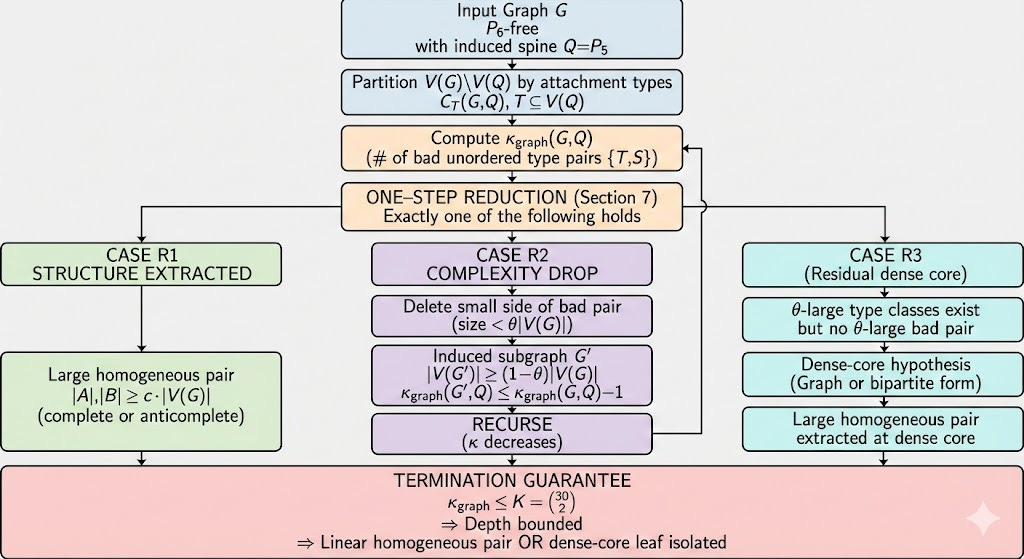
8. One-step reduction: the trichotomy that actually holds
For a P₆-free graph, exactly one of the following happens:
A linear homogeneous pair can be extracted immediately.
A small attachment class from a bad pair can be deleted, reducing κ₍graph₎ while keeping almost all vertices.
You are in the residual regime:
at most one attachment type is θ-large,
there is no θ-large bad pair.
Everything except the third case is handled mechanically.
There is no hidden miracle step. The reduction is explicit and bounded.
9. The bounded-depth theorem
Because κ₍graph₎ starts ≤ 435 and drops by at least one whenever case (2) occurs, the reduction has bounded depth.
After at most K induced restrictions — each losing only a θ-fraction of vertices — the process terminates. Either a linear homogeneous pair has been found, or the graph lies in the residual regime.
This is an unconditional structural theorem.
10. The dense core: the only thing not resolved
What does the residual regime look like?
It is a dense mixed cut between two large attachment classes where:
the cut is neither complete nor empty,
directed degree and codegree are unbounded in both directions.
Local sparsity arguments fail here by construction. This is not a bug. It is the point.
The paper isolates this configuration as the only remaining obstruction to strong Erdős–Hajnal for P₆-free graphs.
11. Bipartite shadows: reframing the hard leaf
Once you are in the dense core, the spine is no longer doing work. What matters is the induced bipartite graph between the two large type classes.
This leads to the notion of a shadow.
The dense-core hypothesis can be reformulated as a strong Erdős–Hajnal statement for a hereditary class of bipartite graphs arising as such shadows.
This reframing matters. It turns a path-theoretic problem into a sharply defined extremal bipartite problem.
12. Why this matters
The reduction is complete. It does not rely on unproven regularity lemmas, probabilistic guesses, or asymptotic hand-waving. Every step is finite, checkable, and monotone.
What remains is not vague: it is a single dense bipartite extraction problem. Either that problem yields to known extremal methods, or it becomes the precise location where P₆-free graphs differ fundamentally from simpler hereditary classes.
In either case, the fog is gone.
There is only one leaf left — and now we know exactly where it is.